Now we will talk about how to represent series of numbers in a visual form using graphs and charts in Excel.

What are graphs and charts in Excel for? Imagine that you are preparing for a speech or writing a report. It’s just that dry numbers will look much worse than the same numbers presented with bright and colorful images.

By using graphs and charts in Excel You can convincingly demonstrate the benefits of your project, show the results of your work, or the work of an entire enterprise, or demonstrate the operation of a machine or mechanism.

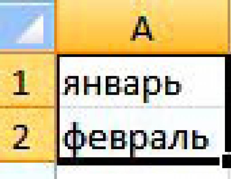
Let's go straight to practice. Let there be a number of figures that characterize the activity of the enterprise for each month during the year. Write in a cell A1 - January, in cell A2 - February. Then select both of these cells, move the cursor to the point in the lower right corner of the selected range, and drag the cursor with the left mouse button pressed to the cell A12. You will have a series of months from January to December.

Now in cells from B1 to B12 write some numbers.

Select a menu item Insert, then select the kind of Excel chart you want to use. There are a lot of options: histogram, graph, pie, bar . In principle, you can iterate through them all in turn: each Excel chart will display the given numbers in its own way.

For example, select one of the chart types Schedule. An empty window will appear. Now click on the icon Select data , and highlight your cells with numbers. Click OK. That, in fact, is all, the schedule will be created.

Graph in Excel can be made much more interesting than it looks now. For example, below are the numbers. But what if you want the names of the months to be displayed under the horizontal axis? To do so, click on Select data , above the window Horizontal axis labels press the button Change, and select the cells with the names of the months. Click OK .

Now let's rename the element Row1, which is below the graph, to something more specific. Click again on Select data , and above the window Legend elements press the button Change. Write the row name in the box, for example: Data for 2012 . Click OK .

Basically, the element Row1 you can generally remove it so that it is not visible in the table if you do not need it. Select it and delete it with the button Delete .

Now fill in the cells with numbers from C1 before C12. Click on the table box. You will see that the column cells B marked with a blue frame. This means that these cells are used in the Excel chart. Drag the corner of the blue frame so that the frame also covers the cells of the column C. You will see that the graph has changed: another curve has appeared. This way we can choose any range of numbers to display in the Excel chart.

Each element Excel charts(curves, chart box, vertical and horizontal axis numbers) can be formatted. To do this, select the appropriate element, right-click on it, and select Data series format .

In addition, if you double-click on the diagram, that is, you get to its editing, you can, in addition to the original data, change Excel chart layout and style. There are a lot of options there - you just need to click on the scroll sliders to the right of these items. You can also move the Excel chart to a separate sheet if desired.

The question remains: how to show on a chart in Excel dependent data series ? For this, the chart type is used dotted. First, write rows of numbers into the cells: in the first column, a row of numbers that will be on the horizontal axis, and in the second column - a row of dependent numbers corresponding to the first column - they will be displayed on the vertical axis. Then choose one of the Excel scatter charts, highlight those columns, and you're done.

You can get more detailed information in the sections "All courses" and "Utility", which can be accessed through the top menu of the site. In these sections, the articles are grouped by subject into blocks containing the most detailed (as far as possible) information on various topics.

You can also subscribe to the blog, and learn about all the new articles.
It does not take a lot of time. Just click on the link below:

Plotting a function in Excel is not a difficult topic and Excel can handle it without problems. The main thing is to set the parameters correctly and choose the appropriate diagram. In this example, we will build a scatter plot in Excel.

Considering that the function is the dependence of one parameter on another, we set the values ​​for the x-axis with a step of 0.5. We will build a graph on the segment [-3; 3]. We call the column "x", write the first value "-3", the second - "-2.5". Select them and drag down the black cross in the lower right corner of the cell.

We will plot a function of the form y=x^3+2x^2+2. In cell B1 we write "y", for convenience, you can enter the entire formula. Select cell B2, put "=" and write the formula in the "Formula Bar": instead of "x" we put a link to the desired cell, to raise the number to a power, press "Shift + 6". When you're done, press "Enter" and drag the formula down.

We have a table, in one column of which the values ​​​​of the argument are written - "x", in the other - the values ​​\u200b\u200bof the given function are calculated.

Let's move on to plotting a function graph in Excel. Select the values ​​for "x" and for "y", go to the tab "Insert" and in the group "Charts" click on the button "Point". Choose one of the proposed types.

The graph of the function looks like this.

Now let's show that the x-axis has a step of 0.5. Select it and right-click on it. Select Axis Format from the context menu.

The corresponding dialog box will open. On the Axis Options tab, in the field "price of major divisions", put a marker in the paragraph "fixed" and enter the value "0.5".

To add a chart title and axis title, turn off the legend, add a grid, fill it, or select an outline, click the Design, Layout, Format tabs.

You can also build a graph of a function in Excel using "Graphics". You can read about how to build a graph in Excel by clicking on the link.

Let's add another graph to this chart. This time the function will look like: y1=2*x+5. We name the column and calculate the formula for different values ​​\u200b\u200bof "x".

Select the diagram, right-click on it and select from the context menu "Select data".

In field "Elements of a Legend" click on the "Add" button.

A window will appear "Row Change". Place the cursor in the "Row Name" field and select cell C1. For the fields "Values ​​X" and "Values ​​Y" select the data from the corresponding columns. Click OK.

So that for the first chart in the Legend it was not written "Row 1", select it and click on the button "Edit".

We put the cursor in the "Row name" field and select the desired cell with the mouse. Click OK.

You can also enter data from the keyboard, but in this case, if you change the data in cell B1, the label on the chart will not change.

The result is the following diagram, on which two graphs are built: for "y" and "y1".

I think now you can build a graph of a function in Excel, and, if necessary, add the necessary graphs to the diagram.

Rate article:

Example 1

Given a function:

It is necessary to build its graph on the interval [-5; 5] with a step equal to 1.

Create a table

Let's create a table, the first column will be called a variable x(cell A1), the second is a variable y(cell B1). For convenience, we will write the function itself in cell B1 so that it is clear which graph we will build. Enter the values ​​-5, -4 in cells A2 and A3 respectively, select both cells and copy them down. We get a sequence from -5 to 5 with a step of 1.

Calculating Function Values

It is necessary to calculate the values ​​of the function at these points. To do this, in cell B2 we will create a formula corresponding to the given function, but instead of x we ​​will enter the value of the variable x, located in the cell on the left (-5).

Important: sign is used for exponentiation ^ , which can be accessed with a keyboard shortcut Shift+6 on the English keyboard layout. Be sure to put a multiplication sign between the coefficients and the variable * (Shift+8).

We complete the entry of the formula by pressing the key Enter. We will get the value of the function at the point x=-5. Copy the resulting formula down.

We got a sequence of function values ​​at points on the interval [-5;5] with a step of 1.

Plotting

Let's select the range of values ​​of the variable x and the function y. Let's go to the tab Insert and in the group Diagrams choose dotted(you can choose any of the scatter plots, but it is better to use the view with smooth curves).

We have obtained the graph of this function. Using tabs Constructor, Layout, Format, You can change the graph settings.

Example 2

Given functions:

andy=50 x+2. It is necessary to build graphs of these functions in one coordinate system.

Creating a table and calculating function values

We have already built a table for the first function, let's add the third column — the values ​​of the function y=50x+2 on the same interval [-5;5]. Fill in the values ​​of this function. To do this, in cell C2 we enter the formula corresponding to the function, but instead of x we ​​take the value -5, i.e. cell A2. Copy the formula down.

We got a table of values ​​for the variable x and both functions at these points.

Plotting

To build graphs, select the values ​​of three columns, on the tab Insert in a group Diagrams choose dotted.

We got graphs of functions in one coordinate system. Using tabs Constructor, Layout, Format, you can change the graph settings.

The last example is convenient to use if you need to find the intersection points of functions using graphs. In this case, you can change the values ​​of the x variable, choose a different interval, or take a different step (less or more than 1). In this case, columns B and C do not need to be changed, the diagram too. All changes will take place immediately after entering other values ​​of the variable x. Such a table is dynamic.

Excel is great at building any graphs and charts.

How to build a graph in Excel 2007

For example, let's build a graph of the function y=x(√x-3) on the segment .
We create a table with two columns. In the first column we will have the values ​​of the argument, and in the second we will have the calculated values ​​of the function. The argument column is filled with values ​​on a given interval with a step of 0.5. And in the cell R3C2 of the function column, we put the formula for its calculation.

After pressing Enter in cell R3C2, the value of the function will be calculated. Let's make this cell active again and move the cursor to the lower right corner so that it changes its appearance to a black cross. Click the mouse and move the cursor down to the last line of the plate. This will copy the formula to all cells.

We got a table filled with function values. Select the cells of the column with its values ​​and go to the "Insert" tab of the top panel.


We press the "Graph" button, select any type that suits us, and we get the graph.


Everything is fine with the Y-axis, but the X-axis contains not the values ​​of the argument, but the numbers of the points. To fix this, right-click on it - "Select Data".


Click on the button that changes the labels of the horizontal axis and select the range with the argument values.


Now our schedule has acquired the proper form.

How to do it in Excel 2003

The beginning is the same, but we can call the diagram wizard by selecting the "Charts" item in the "Insert" menu.


This wizard sets the type and appearance of the future chart, as well as the labels of the axes.
Conquer Excel and see you soon!

Graphs are a good way to analyze information. Typically, they are needed when you want to distinguish between some business data showing the amount of a company's profit for the year, or scientific data showing, for example, how the temperature changes in each month in a certain place. Using Microsoft Excel for charting is a great way to make charts that look professional at work or school. However, not everyone knows how graphs are plotted in Excel. The following is a brief description of the steps to follow to create a chart in this editor. Various other plots that can be created - lines, histograms - are done in a similar way. This example is in Microsoft Excel 2007 for Windows.

So, to get started, open the Excel 2007 editor on your computer. Enter the desired data category for the information you want to compare by placing it in different columns. Each category must be entered in a separate cell, starting with A2. The example in this article creates a graph in Excel that shows fuel, clothing, and entertainment costs.

Then you must make the x-axis labels in row 1. Each label should be in a separate cell, starting with B1. For example, in the case of systematization of expenses, you can select four months.

Enter the required values ​​for the Y-axis in the required cells. The data must match the x-axis and category information. In this example, you can note the amount of money spent on each item for each month, rounding the amounts to a convenient value.

Highlight the entered information in the table by clicking in the upper left corner of the table, and then dragging the mark with the mouse over the entire range of data.

Click on the "Insert" tab in the menu located at the top of the screen. This item will be located in the second tab on the left side.

Choose the type of chart you want to use to represent your data when creating a graph in Excel. For the above data, a histogram is best because it shows well the different x-axis variables that represent different data. Keep in mind that data is displayed differently depending on the type of graph. These varieties are listed in the center of the menu. There is a choice of speakers, linear, and more. In the drop-down menu of structures, the histogram will be displayed after clicking on the corresponding item.

Choose the chart type that best suits the data you've plotted in Excel. When you place the cursor on the corresponding option, you will see its description. For example, selecting "2D Chart" will display it in the appropriate form in your spreadsheet.

Click on the chart you created in Excel and then on the Layout tab. To add a title to the entire chart or its axes, simply click on the "Labels" tab. A drop-down menu will open from which you can select the required options. Make changes as needed in the names, fonts by clicking on the text and performing subsequent editing.

Once you've formatted and edited your chart, you can copy and paste it into other documents. If the copy and paste functions don't work, you can always try to take a screenshot and paste the created graphs in Excel 2007 into any selected document as an image.